Elliptic curves
This post contains content from Andrea Corbellini’s gentle introduction to ECC, which is available under the CC BY 4.0.
Definition
For the purposes of crytography, an elliptic curve is given by the equation \(y^3 = x^2 + ax+ b\), subject to \(4a^3 + 27b^2 \neq 0\) (the discriminant). The constraint is applied to exclude points of singularity (where the curve is not well-behaved, for example, not differentiable).
Plotting elliptic curves
Python’s matplotlib and numpy make this extremely easy.
1
2
3
4
5
6
7
8
9
10
11
12
13
14
15
16
17
18
19
20
21
22
23
24
# Choose ranges and # of points for x and y
y, x = np.ogrid[ -5:5:1000j, -2.5:3.5:1000j ]
# Decide the parameters of the curve
b = 2
for a in range( 0, -4, -1 ):
    # Set up the equation
    plt.contour(
        x.ravel(),
        y.ravel(),
        pow( y, 2 ) - pow( x, 3 ) - x * a - b,
        [ 0 ],
    )
    # Show the grid
    plt.grid()
    # Add the label
    plt.text(
        0, 4, f"a = {a}",
        bbox = dict( facecolor = 'black', alpha = 0.8 ),
        color = 'white',
    )
    # Save it
    plt.savefig( f"a={a}.png", dpi = 300, bbox_inches = 'tight' )
    # Plot it
    plt.show()
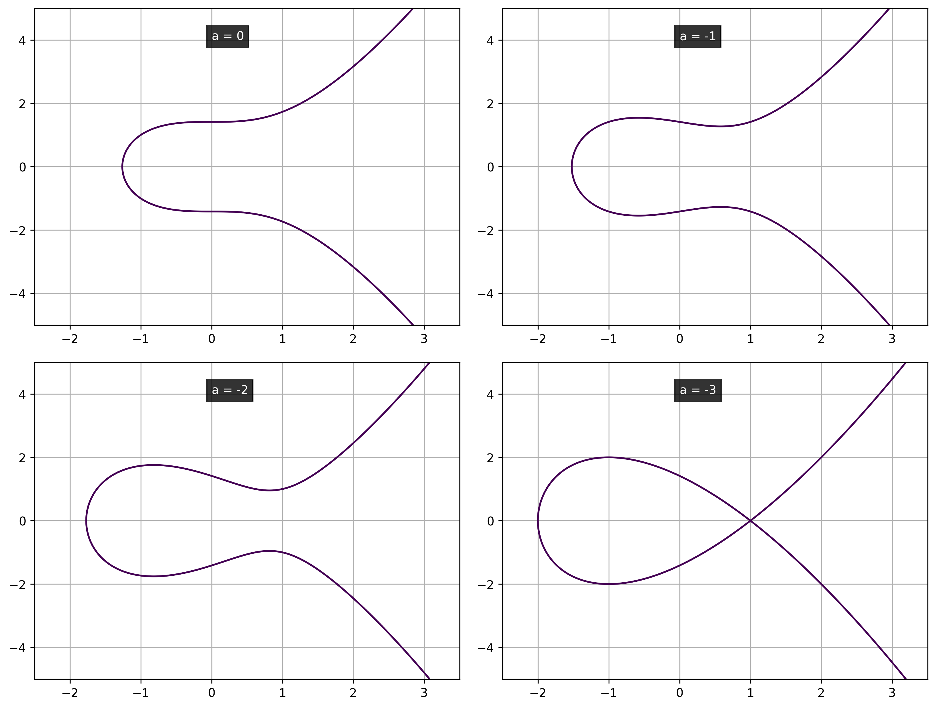
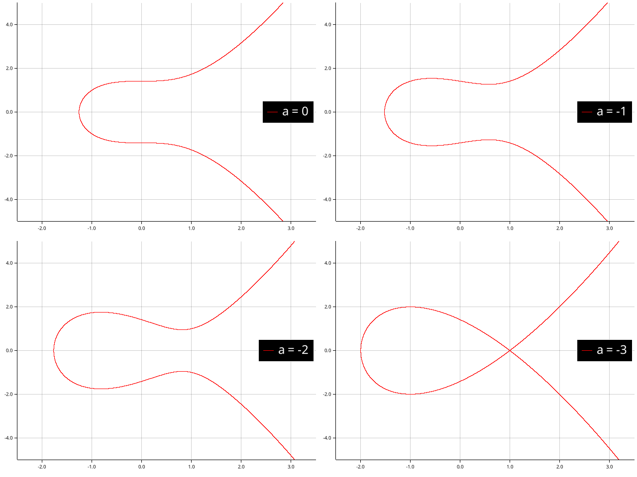
Of these, note that the curve which intersects with itself (\(a = -3\)) is not a valid elliptic curve for our purposes (\(4a^3 + 27b^2 = 4(-3)^3 + 27(2)^2 = 0\)). This is because, at the point of the intersection, the curve is not differentiable.

Generating these images in Rust is a bit more involved because you have to set up the points yourself. This makes the plotters library a little more powerful because it “is a drawing library rather than a traditional data plotting library”.
1
2
3
4
5
6
7
8
9
10
11
12
13
14
15
16
17
18
19
20
21
22
23
24
25
26
27
28
29
30
31
32
33
34
35
36
37
38
39
40
41
42
43
44
45
46
47
48
49
50
51
52
53
54
55
56
57
58
59
60
61
62
63
64
65
66
67
68
69
// tested with 0.3.5
use plotters::prelude::*;

fn main() -> Result<(), Box<dyn std::error::Error>> {
    let b = 2.0;
    for a in (-3..=0).rev() {
        let path = format!("data/a={}.png", a);
        // canvas
        let root =
            BitMapBackend::new(&path, (640, 480)).into_drawing_area();
        root.fill(&WHITE)?;

        // chart configuration within canvas
        let mut chart = ChartBuilder::on(&root)
            .margin(5)
            .x_label_area_size(30)
            .y_label_area_size(30)
            .build_cartesian_2d(-2.5..3.5, -5.0..5.0)?;

        // gridlines
        chart
            .configure_mesh()
            .x_labels(6)
            .y_labels(5)
            .max_light_lines(0)
            .draw()?;

        // data estimation
        let base = 10_000_000f64;
        let mut pos = Vec::new();
        for z in (-2.5 * base) as i32..=(3.5 * base) as i32 {
            let x = z as f64 / base;
            let rhs = x.powi(3) + (x * (a as f64)) + b;
            if rhs < 0.0 {
                continue;
            }
            let y = rhs.sqrt();
            if y > 5.0 {
                break;
            }
            pos.push((x, y));
        }

        chart
            .draw_series(LineSeries::new(
                pos.iter().map(|&(x, y)| (x, y)),
                &RED,
            ))?
            .label(format!("a = {}", a))
            .legend(|(x, y)| {
                PathElement::new(vec![(x, y), (x + 20, y)], &RED)
            });
        chart.draw_series(LineSeries::new(
            pos.iter().map(|&(x, y)| (x, -y)),
            &RED,
        ))?;

        chart
            .configure_series_labels()
            .border_style(&WHITE)
            .background_style(&BLACK)
            .label_font(("Calibri", 30).with_color(&WHITE))
            .draw()?;

        root.present()?;
    }

    Ok(())
}

Besides the curve, we also include the point at infinity \({0}\), which is the equivalent of zero in point arithmetic. It is not a point on the graph - just the identity of the elliptic curve group.
Groups
Groups may seem to be a bit of a digression from the topic of elliptic curves, but they are not. A group \(\mathbb{G}\) is a set for which a binary operation \(+\) called addition is defined in such a manner that it respects the following properties.
- closure: if \(a, b \in \mathbb{G}\) then \(a + b \in \mathbb{G}\)
- associativity: \((a + b) + c = a + (b + c)\)
- identity: \(\exists\text{ }0 \in \mathbb{G} \mid a + 0 = 0 + a = a\)
- inverse: \(\forall\text{ }a \in \mathbb{G}\text{ }\exists\text{ }b \in \mathbb{G} \mid a + b = 0\)
An Abelian group has the additional property of commutativity, that is, \(a + b = b + a \text{ }\forall\text{ }a, b \in \mathbb{G}\).
Examples of groups include the set of integers \(\mathbb{I}\) and the set of real numbers \(\mathbb{R}\), but not the set of natural numbers \(\mathbb{N}\), which does not satisfy the presence of identity property. Similarly the set of whole numbers \(\mathbb{W}\) is excluded because it does not satisfy the presence of inverse property
Addition over elliptic curves
A group over elliptic curves can be defined by defining addition, the identity element and the inverse of an element.
- The identity element, as previously mentioned, is the point at infinity \(0\).
- Addition is defined for three collinear points \(P, Q, R\) lying on the curve as \(P + Q + R = 0\). Since this addition only requires three collinear points and collinearity is without order, it satisfies the properties of both associativity and commutativity.
- The inverse of an element \(A = (x_0, y_0)\) is the one mirrored by the x-axis \(-A = (x_0, -y_0)\).
Addition using geometry
If \(P + Q + R = 0\), it means \(P + Q = -R\). In other words, if we draw a line intersecting the curve at three points, the additive inverse of the any two points is the point symmetric about the x-axis to the third point.
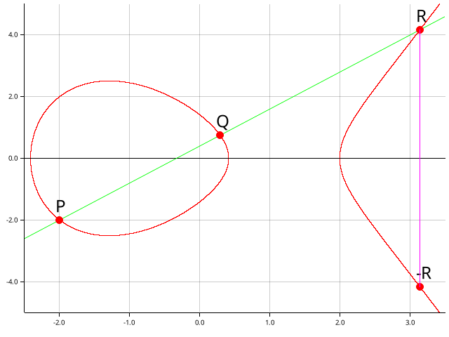
Here’s an example demonstrating the process (of both plotting the example and solving for \(R\)), with the line being plotted as passing through \((-2, -2)\) (which is on the curve) and \((3, 4)\). The line’s equation is
\[y - 4 = \frac{4-(-2)}{3-(-2)}(x - 3), or\\ y = 1.2x + 0.4\]We can substitute the value of \(y\) into the curve’s equation.
\[y^2 = x^3 - 5x + 2\text{ and }y = 1.2x + 0.4\\ (1.2x + 0.4)^2 = x^3 - 5x + 2\\ 1.44x^2 + 0.16 + 0.96x = x^3 - 5x + 2\\ x^3 - 1.44x^2 - 5.96x + 1.84 = 0\\ 25x^3 - 36x^2 - 149x + 46 = 0\]We know from before that \(x = -2\) is a solution to this equation. Even if we didn’t - the last term of this equation is \(46\), and if the equation has any integer roots, they are factors of this number. We can bruteforce through this list: \(\pm 1, \pm 2, \pm 23, \pm 46\). Knowing that, we can say that \(x + 2\) is a factor of \(25x^3 - 36x^2 - 149x + 46 = 0\)
Dividing the polynomial by the factor, we get \(25x^2 - 86x + 23 = 0\), whose roots can be determined using the quadratic formula.
\[x = \frac{86 \pm \sqrt{86^2 - 4(25)(23)}}{2(25)}\\ x = \frac{86 \pm \sqrt{5096}}{2(25)}\\ x = \frac{43 \pm \sqrt{1274}}{25}\\ x = \frac{43 \pm 7\sqrt{26}}{25}\]At these points, y is
\[y = 1.2x + 0.4 y = \frac{6}{5}\frac{43 \pm 7\sqrt{26}}{25} + \frac{2}{5} y = \frac{306 \pm 42\sqrt{26}}{125}\]For any two points \(P, Q\) on the line and the curve, the mirror image of the third point about the x-axis is their sum.
\[P = (-2, -2)\\ Q = (\frac{43 - 7\sqrt{26}}{25}, \frac{306 - 42\sqrt{26}}{125})\\ R = (\frac{43 + 7\sqrt{26}}{25}, \frac{306 + 42\sqrt{26}}{125})\\ P + Q + R = 0\\ P + Q = -R = (x_r, -y_r) = (\frac{43 + 7\sqrt{26}}{25}, \frac{-306 - 42\sqrt{26}}{125})\]This analysis can be plotted similarly in Rust.
1
2
3
4
5
6
7
8
9
10
11
12
13
14
15
16
17
18
19
20
21
22
23
24
25
26
27
28
29
30
31
32
33
34
35
36
37
38
39
40
41
42
43
44
45
46
47
48
49
50
51
52
53
54
55
56
57
58
59
60
61
62
63
64
65
66
67
68
69
70
71
72
73
74
75
76
77
78
79
80
81
82
83
84
85
86
87
88
89
90
91
92
93
94
95
96
97
98
99
100
101
102
103
104
105
106
107
108
109
110
111
112
113
114
115
116
117
118
119
let b = 2.0;
let a = -5;
let path = "data/addition.png";
// canvas
let root =
    BitMapBackend::new(&path, (640, 480)).into_drawing_area();
root.fill(&WHITE)?;

// chart configuration within canvas
let mut chart = ChartBuilder::on(&root)
    .margin(5)
    .x_label_area_size(30)
    .y_label_area_size(30)
    .build_cartesian_2d(-2.5..3.5, -5.0..5.0)?;

// gridlines
chart
    .configure_mesh()
    .x_labels(6)
    .y_labels(5)
    .max_light_lines(0)
    .draw()?;

// data estimation
let base = 10_000_000f64;
let mut pos = Vec::new();
for z in (-2.5 * base) as i32..=(3.5 * base) as i32 {
    let x = z as f64 / base;
    let rhs = x.powi(3) + (x * (a as f64)) + b;
    if rhs < 0.0 {
        continue;
    }
    let y = rhs.sqrt();
    if y > 5.0 {
        break;
    }
    pos.push((x, y));
}

chart
    .draw_series(LineSeries::new(
        pos.iter().map(|&(x, y)| (x, y)),
        &RED,
    ))?
    .label(format!("a = {}", a))
    .legend(|(x, y)| {
        PathElement::new(vec![(x, y), (x + 20, y)], &RED)
    });
chart.draw_series(LineSeries::new(
    pos.iter().map(|&(x, y)| (x, -y)),
    &RED,
))?;

// y = 0 is drawn after (on top of) the curve
// because plotters is automatically
// joining the two consecutive
// points with y = 0
chart.draw_series(LineSeries::new(
    [(-2.5f64, 0f64), (3.5f64, 0f64)],
    &BLACK,
))?;

// we draw this line over the range of x to make it look complete
// this line is y - 4.6 = 1.2( x - 3.5 ) or y - 0.4 = 1.2x
chart.draw_series(LineSeries::new(
    [(-2.5f64, -2.6f64), (3.5f64, 4.6f64)],
    &GREEN,
))?;

// substitute the equation for y in the curve
// 25x^3 - 36x^2 - 149x + 46 = 0
// the line touches the curve at (-2, -2)
// so divide that polynomial by x + 2
// which gives 25x^2 - 86x + 23 = 0
// that can easily be solved using the quadratic formula
let xs = [
    // increasing order of x coordinates
    -2f64,
    (43f64 - 7f64 * (26 as f64).sqrt()) / 25f64,
    (43f64 + 7f64 * (26 as f64).sqrt()) / 25f64,
];
let point_labels = ["P", "Q", "R"];
chart.draw_series(PointSeries::of_element(
    xs.iter().map(|&x| (x, 1.2 * x + 0.4)),
    5,
    &RED,
    &|c, s, st| {
        return EmptyElement::at(c)
            + Circle::new((0, 0), s, st.filled())
            + Text::new(
                point_labels
                    [xs.iter().position(|&r| r == c.0).unwrap()],
                (-5, -30),
                ("sans-serif", 30).into_font(),
            );
    },
))?;
let r_pos = point_labels.iter().position(|&c| c == "R").unwrap();
let r = (xs[r_pos], 1.2 * xs[r_pos] + 0.4);
chart.draw_series(PointSeries::of_element(
    [(r.0, -r.1)],
    5,
    &RED,
    &|c, s, st| {
        return EmptyElement::at(c)
            + Circle::new((0, 0), s, st.filled())
            + Text::new(
                "-R",
                (-5, -30),
                ("sans-serif", 30).into_font(),
            );
    },
))?;
let r_line = [(r.0, r.1), (r.0, -r.1)];
chart.draw_series(LineSeries::new(r_line, &MAGENTA))?;

root.present()?;

Ok(())

Selected cases when considering addition
If either \(P = 0\) (or \(Q = 0\)), we can say that \(P + Q = P + 0 = P\) (or \(P + Q = 0 + Q = Q\)) by the definition of the identity element of the group.
If \(P = -Q\), then there is only one line passing via the points P and Q, which are symmetric about the x-axis. This means, again by definition, that \(P + Q = 0\).
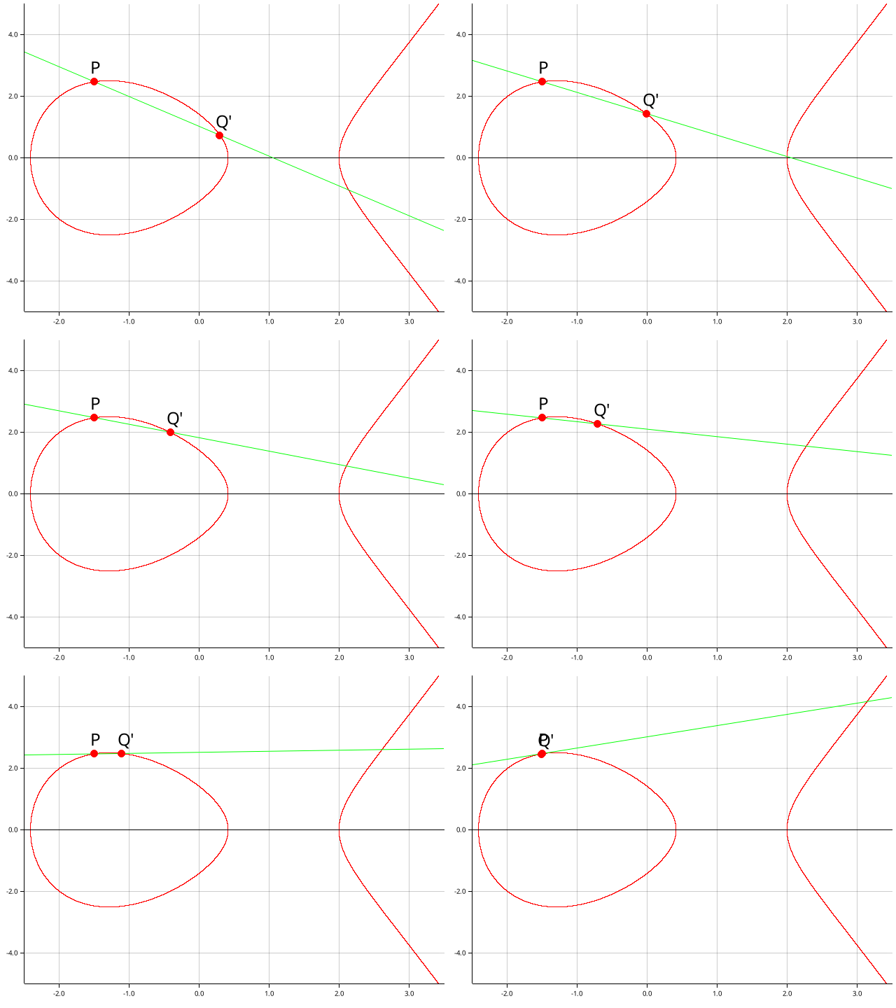
If \(P = Q\), then it gets a bit trickier. There are infinite lines passing via such a point (and obviously, the curve). I like to think of this using limits: consider a point \(Q' \ne P\). What happens if we make \(Q'\) move closer to \(P\), till they coincide?

Each frame of this GIF was generated one-by-one, and then merged.
1
2
3
4
5
6
7
8
9
10
11
12
13
14
15
16
17
18
19
20
21
22
23
24
25
26
27
28
29
30
31
32
33
34
35
36
37
38
39
40
41
42
43
44
45
46
47
48
49
50
51
52
53
54
55
56
57
58
59
60
61
62
63
64
65
66
67
68
69
70
71
72
73
74
75
76
77
78
79
80
81
82
83
84
85
86
87
88
89
90
91
92
93
94
95
96
97
98
99
100
101
102
103
104
105
106
107
108
109
110
111
112
113
114
115
116
117
118
119
120
121
122
123
124
125
126
127
128
129
// curve parameters
let b = 2.0;
let a = -5;
let y_sign = 1f64;
// data estimation parameters
let base = 10_000_000f64;
let step = 1_000_000;
// graph parameters
let x_range = (-2.5, 3.5);
let y_range = (-5.0, 5.0);
// starting points P and Q chosen so that
// everything fits in the bounds
// these are for demonstration only
// the example is valid for any points
let p = (-1.5f64, 6.125_f64.sqrt() * y_sign);
let mut q = (
    (43f64 - 7f64 * (26 as f64).sqrt()) / 25f64,
    (306f64 - 42f64 * (26 as f64).sqrt()) * y_sign / 125f64,
);
// data estimation
let mut pos = Vec::new();
for z in (x_range.0 * base) as i32..=(x_range.1 * base) as i32 {
    let x = z as f64 / base;
    let rhs = x.powi(3) + (x * (a as f64)) + b;
    if rhs < 0.0 {
        continue;
    }
    let y = rhs.sqrt();
    if y > y_range.1 {
        break;
    }
    pos.push((x, y));
}
// loop counter
let mut index = -1;
// we re-draw the curve each frame
// and reduce q_x by decrease/base, and find the corresponding y
while p.0 < q.0 || p.0 - q.0 <= (step as f64) / base {
    // canvas
    index = index + 1;
    let path = format!("data/tangent_{}.png", index);
    println!("{}", path);
    let root =
        BitMapBackend::new(&path, (640, 480)).into_drawing_area();
    root.fill(&WHITE)?;

    // chart configuration
    let mut chart = ChartBuilder::on(&root)
        .margin(5)
        .x_label_area_size(30)
        .y_label_area_size(30)
        .build_cartesian_2d(
            x_range.0..x_range.1,
            y_range.0..y_range.1,
        )?;

    // gridlines
    chart
        .configure_mesh()
        .x_labels(6)
        .y_labels(5)
        .max_light_lines(0)
        .draw()?;

    // positive data of curve
    chart
        .draw_series(LineSeries::new(
            pos.iter().map(|&(x, y)| (x, y)),
            &RED,
        ))?
        .label(format!("a = {}", a))
        .legend(|(x, y)| {
            PathElement::new(vec![(x, y), (x + 20, y)], &RED)
        });
    // negative data of curve
    chart.draw_series(LineSeries::new(
        pos.iter().map(|&(x, y)| (x, -y)),
        &RED,
    ))?;

    // y = 0 line to work around plotters automatic joining
    chart.draw_series(LineSeries::new(
        [(x_range.0, 0f64), (x_range.1, 0f64)],
        &BLACK,
    ))?;

    // widest line passing through points P and Q
    let slope = (q.1 - p.1) / (q.0 - p.0);
    let line = [
        (x_range.0, p.1 + slope * (x_range.0 - p.0)),
        (x_range.1, p.1 + slope * (x_range.1 - p.0)),
    ];
    chart.draw_series(LineSeries::new(line, &GREEN))?;

    // draw the points P and Q, on top of the line
    let points = [p, q];
    let point_labels = ["P", "Q'"];
    chart.draw_series(PointSeries::of_element(
        points,
        5,
        &RED,
        &|c, s, st| {
            return EmptyElement::at(c)
                + Circle::new((0, 0), s, st.filled())
                + Text::new(
                    point_labels[points
                        .iter()
                        .position(|&r| r == c)
                        .unwrap()],
                    (-5, -30),
                    ("sans-serif", 30).into_font(),
                );
        },
    ))?;

    // dump chart
    root.present()?;

    // find the first element < q_x in pos
    q = match pos.iter().step_by(step).rev().find(|(x, _)| x < &q.0)
    {
        Some((x, y)) => (*x, y_sign * *y),
        None => {
            break;
        }
    };
}

Ok(())
The line that passes through P is tangent to the curve and intersects the curve at R such that \(P + P + R = 0,\text{ or, }2P = -R\). In other words, the cubic equation (in \(x\)) resulting from the intersection of the curve and the line has two equal roots (\(x_p\) twice).
The observation, that the line is tangent to P, which we made with the GIF above can be made algebraically by calculating the slope of the line \(PQ'\) when \(Q'\) is extremely close to \(P\). This is, obviously, equal to the slope of the curve at \(P\).
\[P = (x_p, y_p)\\ Q' = (x_q, y_q)\\ m = \frac{y_q-y_p}{x_q-x_p}\\ \lim\limits_{Q' \rarr P} m = \frac{dy}{dx}\mid_{(x_p, y_p)} = \frac{3x^2_p - 5}{5y_p}\]If \(P \ne Q\) and the line does not touch the curve again, the case is similar to the previous one. The line passing through \(P\) and \(Q\) is tangent to the curve. If the line is tangent to the curve at \(P\), it means \(2P + Q = 0\); if it is tangent at line \(Q\), then \(2Q + P = 0\).
Algebraic addition
As I demonstrated above, solving the equation for a line and its intersection with the elliptic curve isn’t quick because of the cubic nature of the equations. But there is a way out. Let there be two points \(P (x_p, y_p)\) and \(Q (x_q, y_q)\) such that \(x_p \ne x_q\). The slope \(m\) of the line \(PQ\) can be calculated.
\[m = \frac{y_q - y_p}{x_q - x_p}\]The line’s equation \(y - y_p = m(x - x_p)\) can be substituted into the curve to find \((x_r, y_r)\).
\[y^2 = x^3 + ax + b\\ (y_p + m(x-x_p))^2 = x^3 + ax + b\\ y^2_p + m^2(x-x_p)^2 + 2my_p(x-x_p) = x^3 + ax + b\\ y^2_p + m^2(x^2 + x^2_p - 2xx_p) + 2my_p(x - x_p) = x^3 + ax + b\\ y^2_p + m^2x^2 + m^2x^2_p - 2m^2xx_p + 2my_px - 2my_px_p = x^3 + ax + b\\ x^3 - m^2x^2 + x(a + 2m^2x_p - 2my_p) + (b - m^2x^2_p + 2mx_py_p - y^2_p) = 0\]This equation has three roots \(x_p, x_q, x_r\), the sum of which is equal to \(m^2\).
\[x_p + x_q + x_r = m^2\\ x_r = m^2 - x_p - x_q\\ y_r = m(x_r - x_p) + y_p \text{ or } y_r = m(x_r - x_q) + y_q\]Scalar multiplication
Besides addition of two points, we can define scalar multiplication.
\[nP = \underbrace{P + P + ... + P}_{\text{n times}}\]Written this way, it appears to take \(O(n)\) time which is not very fast. A faster algorithm is the double and add method. It requires decomposing a number into \(k\) bits and adding them up similar to a traditional binary conversion. This algorithm is \(O(\log n)\) or \(O(k)\).
\[250 = 2^71 + 2^61 + 2^51 + 2^41 + 2^31 + 2^20 + 2^11 + 2^00\\ 250 = 2^7 + 2^6 + 2^5 + 2^4 + 2^3 + 2^1\\ 250 = (11111010)_2\]This means, \(250P\) can be calculated similarly.
\[250 = 2^7P + 2^6P + 2^5P + 2^4P + 2^3P + 2^1P\]- Double \(P\), and store it as the sum (\(2^1P\)).
- Double \(P\) again, and do not add it to the sum (\(2^1P\)).
- Double it again, and add it to the sum (\(2^1P + 2^3P\)).
- ….
In the end, we are able to compute \(250P\) via 7 doublings and 6 additions. Assuming that the doublings and the additions are \(O(1)\), the algorithm is \(O(k)\) which is better than step-by-step addition \(O(2^k)\).
Logarithm
The reverse of the above process of scalar multiplication is called logarithm. We use the term logarithm and not division to be congruent with other cryptosystems that use exponentiation instead of multiplication. If \(Q = nP\) given both \(Q\) and \(P\), what is the value of \(n\)?
There may not be a quick way to solve this problem, but it is certainly possible on a case-by-case basis using numerical methods and/or approximation techniques. However, if we change the domain of the elliptic curves from \(\Reals\) to \(\Z_p\) where \(p > 3\) is a prime, the logarithm problem becomes “discrete” and difficult to solve for larger values of \(p\). Here, \(\Reals\) refers to the domain of real numbers and \(\Z_p\) is a prime field.
The duality, that scalar multiplication is “easy” and discrete logarithm is “hard”, is the cornerstone of elliptic curve cryptography.